Introduction to Graph in Programming

The idea for this blog is to discuss another way of storing data i.e. Graph. This is one of the important topics that is asked in the interviews of companies like Google, Facebook, Amazon, etc. So, in this blog, we will be covering the below topics:

• What is a Graph?
• Properties of a Graph
• Types of Graph
• Graph Representation: Adjacency Matrix
• Graph Representation: Adjacency List

So, let's get started with the basics of Graph.

What is a Graph in Data Structure?

In a Graph, we have a set of nodes (a.k.a vertices) and these nodes are connected with each other with the help of some edges. The nodes or vertices are used to store data and this data can be used further.

A graph is a type of non-linear data structure that is used to store data in the form of nodes and edges.

The following is a typical representation of Graph:

G = (V, E) 
Here G is the Graph, V is the set of vertices or nodes and E is the set of edges in the Graph G.

The following is the pictorial representation of a Graph having 5 nodes or vertices:

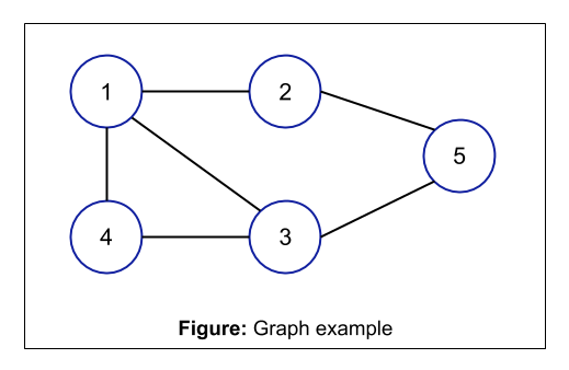
The above is an example of Graph having a set of vertices as V = {1, 2, 3, 4, 5} and the set of edges as E = {1-2, 1-3, 1-4, 2-1, 2-5, 3-1, 3-4, 3-5, 4-1, 4-3, 5-2, 5-3}.

Some of the practical scenarios where we can use the Graph to represent data are:

• Social-Media connections: Here, every user can be represented as a node and the nodes can be connected with each other with the help of some edge.

For example, in the case of Facebook, each user is represented as a node that contains all the information about the users like name, place, id, etc. and the edges between the nodes can be the relationship between the nodes i.e. here the relationship is "Friend". Similarly, in the case of LinkedIn, the nodes are the users and the relationship can be a "Connection" i.e. A is a connection with B.

• Telephone network: In the case of telephone network various nodes or telephones are connected with each other with the help of wires i.e. edges. So, this is an example of a graph.
• Finding routes: Finding the shortest path between two places is a classical example of a Graph. Here, the places are represented as nodes and the possible paths between the nodes are the edges between the nodes.

These are some of the real-life examples of a Graph. Try to find more such examples and make a graph diagram of the same. Let's move further and look at some of the properties of a Graph.

Properties of a Graph

Here in this section of the blog, we will learn some of the properties of a Graph that will be helpful in solving the graph problems:

• Distance between vertices: It is the minimum number of edges present between two nodes. If there are more than one possible paths from one node to another, then the distance between those two vertices is the shortest path between those vertices. It is represented by:

d(A, B); Here, A and B are the nodes and d is the distance between these two nodes

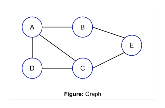
In the above example, the distance between node A and B can be represented as d(A, B) and it is equal to 1 because:

path 1: A -> B, length = 1
path 2: A - > C -> E -> B, length = 3
path 3: A -> D -> C -> A -> B, length = 4
path 4: A -> D -> C -> E -> B, length = 4
Minimum length = 1

• Eccentricity: The eccentricity is defined as the maximum distance between a vertex to all other vertices. It is represented by:

e(V); Here, V is the vertex and e is the eccentricity of V

In the above example, the eccentricity of node A is the maximum distance from A to other vertices i.e. 2

distance between A and B: 1
distance between A and C: 2
distance between A and D: 1
distance between A and E: 2 (because distance is the shortest path)
Maximum distance = 2

• Radius: It is the minimum eccentricity i.e. the minimum distance between a vertex to all the vertices. It is represented by:

r(G); Here G is the connected graph and r is the radius of G

• Diameter: It is the maximum eccentricity i.e. the maximum distance between a vertex to all the vertices. It is represented by:

d(G); Here G is the connected graph and d is the diameter of G

• Central Point: For a vertex, if the eccentricity of the graph is equal to its radius, then that vertex is called the central point of the graph.

e(V) = r(V); Here e is the eccentricity and r is the radius of vertex V

• Circumference: It is the total number of edges that are present in the longest cycle of a graph.

These are some of the properties of a Graph. Let's look at some of the types of Graph.

Types of a Graph

In this part of the blog, we will learn various types of graphs and this will help us in transforming a real-life problem into some graph problem. You will get to know which graph should be used when.

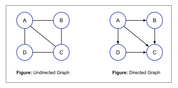
• Directed and Undirected Graph: It is a very basic type of graph. A graph can be directed or undirected i.e. the edges of a graph can be undirected or directed. In an undirected graph, for every edge, you can traverse in both the direction i.e. if there is an edge between node A and node B, then you can traverse from node A to node B or from node B to node A. But in a directed graph, the direction is given to you and you can traverse in the given direction only. For example,

For an undirected graph, the total number of possible edges will be: 
nC2 i.e. (n(n-1))/2
While for a directed graph, the total number of possible edges will be:
2*nC2 i.e. 2(n(n-1))/2 = n(n-1)

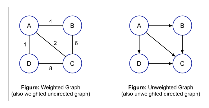
• Weighted and Unweighted Graph: You can assign some weights or costs over an edge of a graph. If there is some weight or cost over the edges of the graph, then it is known as a weighted graph otherwise it is called an unweighted graph.

For example, suppose we are representing the cities of a state as nodes and these nodes are connected with the help of edges. So, here we can put the distance between these cities over the edges i.e. we are putting some weight over the edges of the graph. So, this type of graph is called a weighted graph. If there is no weight on the edges, then it is called an unweighted graph.

• Cyclic and Acyclic Graph: If there is a cycle in a graph then that graph is called Cyclic Graph. A graph is said to have a cycle if you start from a node/vertex and after traversing some nodes, you come to the same node, then you can say that the graph is having a cycle. If there is no cycle present in the graph, then that graph is called an Acyclic Graph. For a Cyclic Graph, at least one cycle is necessary.

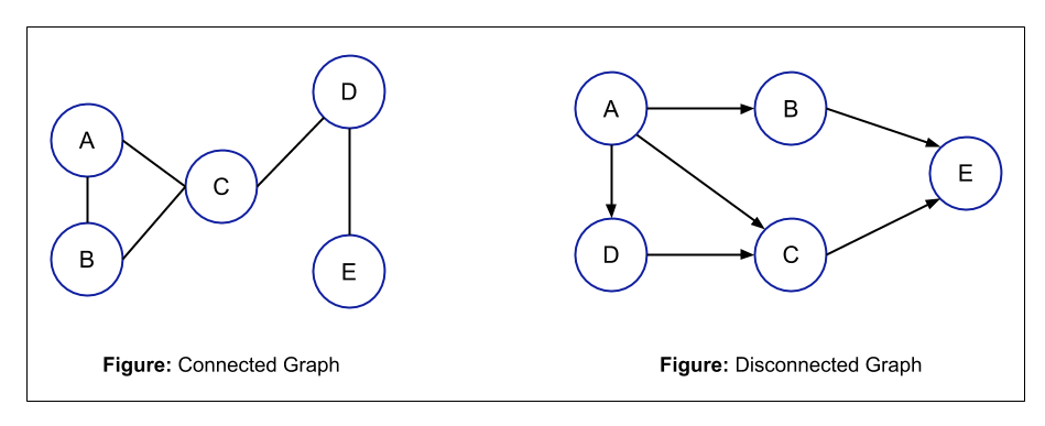
• Connected and Disconnected Graph: In a Connected Graph, from each node, there is a path to all the other nodes i.e. from each node, you can access all the other nodes of the graph. But in a Disconnected Graph, you can't access all the nodes from a particular node.

• Sparse and Dense Graph: If the number of edges of a graph is close to the total number of possible edges of that graph, then the graph is said to be Dense Graph otherwise, it is said to be a Sparse Graph.

For example, if a graph is an undirected graph and there are 5 nodes, then the total number of possible edges will be n(n-1)/2 i.e. 5(5-1)/2 = 10. Now, if the graph contains 4 edges, then the graph is said to be Sparse Graph because 4 is very less than 10 and if the graph contains 8 nodes, then the graph is said to be Dense Graph because 8 is close to 10 i.e. total number of possible edges.

These are some of the types of graphs that we use in data structures.

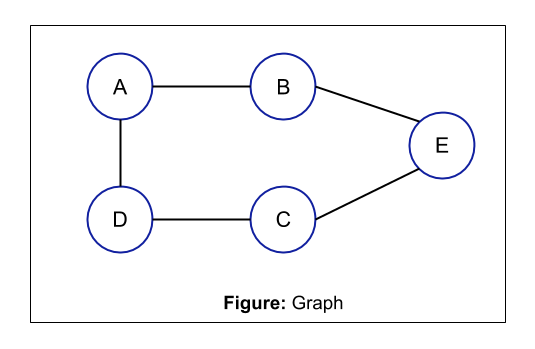
NOTE: A graph can be a combination of more than two or more graphs from the above graph types.

For example:

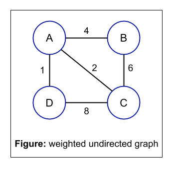
The above image is a combination of a weighted, undirected, cyclic, and dense graph.

Graph Representation

Till now, we have seen the pictorial representation of a graph. But in a programming language, we can't use this pictorial representation to perform various operations on the graph. So, to represent a graph, we use the below two methods:

• Adjacency Matrix
• Adjacency List

Let's learn one by one.

Adjacency Matrix

Let us assume that the graph is G(n, m). Here G is the graph, n is the total number of nodes and m is the total number of edges present in the graph G.

We know that the total number of possible edges of an undirected graph is n(n-1)/2 and that of a directed graph is n(n-1). So, the value of "m" should lie between:

1 <= m <= n(n-1)/2 ------> for undirected graph
1 <= m <= n(n-1)   ------> for directed graph

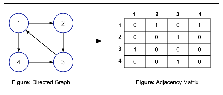
So, we use an Adjacency matrix which is a 2D matrix of size n*n, where n is the number of nodes present in the graph. Also, we will mark each node from 1 to n. In the adjacency matrix, we fill the matrix according to the below rule:

matrix[i][j] = 1; if there is an edge between node i and node j
matrix[i][j] = 0; if there is no edge between node i and node j

Here, the total space used is O(n*n).

For example,

NOTE: For a weighted graph, instead of putting "1" in the matrix, you can put the weight of the edge in the matrix i.e.

matrix[i][j] = weight of the edge between node i and node j

Searching

Now, if you want to find if there is an edge between two nodes of a graph, then you can do this in O(1). For example, if matrix[i][j] == 1, then there is an edge between node i and node j.

Inserting edge

If you want to insert some edge between node i and node j, then all you need to do is just make matrix[i][j] = 1. This operation can be done in O(1).

Deleting edge

If you want to delete some edge between node i and node j, then all you need to do is just make matrix[i][j] = 0. This operation can be done in O(1).

★ In an undirected graph, the path is bidirectional i.e. you can go from node i to node j and vice-versa. So, the adjacency matrix is symmetrical along the diagonal i.e. you can either use the upper part or the lower part of the diagonal. In this way, you can save space while storing the values in the matrix.

Problems with Adjacency Matrix

In an Adjacency matrix, we create a matrix of size n*n, where n is the number of nodes present in the graph. Now, suppose the graph is a Sparse graph i.e. total number of edges present in the graph is very less as compared to the total possible edges.

For example, if the total number of nodes is 5 and the number of edges is 4. Then we will make a matrix of size 5*5 = 25 and we are storing the value of only 4 edges. Rest of the 21 spaces are vacant. So, here there is a waste of memory.

In order to solve this problem of wastage of memory in case of a Sparse matrix, we use the Adjacency List.

Adjacency List

Let us assume that the graph is G(n, m). Here G is the graph, n is the number of nodes and m is the total number of edges present in the graph G.

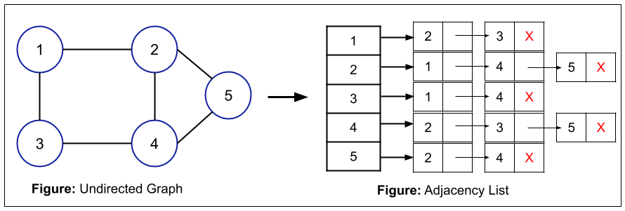
Now, to represent the graph in the form of an Adjacency List, we will create a list of pointers of size "n". Each node in the list denotes the node present in the graph. These nodes are pointing towards a list of nodes that can be traversed from a particular node. All the nodes connected from a particular node are added in the list corresponding to that particular node. For example, if from node A, node B and node C are connected, then the linked list will be A -> B -> C.

In case of an undirected graph, the total number of nodes of the linked list will be 2m (because the connection is bidirectional), where "m" is the number of edges of the graph.

Also, in the case of an undirected graph, the total space used is O(n + 2m).

In case of a directed graph, the total number of nodes of the linked list will be m, where "m" is the number of edges of the graph.

Also, in the case of a directed graph, the total space used is O(n + m).

If you want to add some edge between node i and node j, then you have to first go to matrix[i] and then traverse the whole list corresponding to matrix[i] and add the new edge at the last. Similarly, for deletion of an edge between node i and node j, you have to go to matrix[i] and then find the edge in the linked list corresponding to matrix[i] and then perform the delete operation. So, insertion and deletion are costlier in case of an adjacency list.

Which representation to use when?

• For a Sparse Graph, you should prefer using Adjacency List over the Adjacency Matrix. But for a Dense Graph, you should go with Adjacency Matrix.
• If you frequently need to check if there is an edge present between two nodes or not or you need to add or delete edges frequently, then you should use Adjacency Matrix.

Critical ideas to think

• Find some of the real-life examples that can be converted to some graph problem.
• Find how to traverse a graph i.e. how to visit all the nodes of a graph from a source node.
• Try to make Adjacency Matrix and Adjacency List of a weighted graph.

Happy Learning, Enjoy Algorithms!

Team AfterAcademy!