Process scheduling algorithms in the Operating System
AfterAcademy Tech
•
12 Nov 2019
In a system, there are a number of processes that are present in different states at a particular time. Some processes may be in the waiting state, others may be in the running state and so on. Have you ever thought how CPU selects one process out of some many processes for execution? Yes, you got it right. CPU uses some kind of process scheduling algorithms to select one process for its execution amongst so many processes. The process scheduling algorithms are used to maximize CPU utilization by increasing throughput. In this blog, we will learn about various process scheduling algorithms used by CPU to schedule a process.
But before starting this blog, if you are not familiar with Burst time, Arrival time, Exit time, Response time, Waiting time, Turnaround time, and Throughput, then you should first learn these topics by reading the blog from here. Also, learn about Preemptive and Non-Preemptive scheduling from here.
Since you are done with the prerequisites of this blog, let's get started by learning different process scheduling algorithms.
First Come First Serve (FCFS)
As the name suggests, the process coming first in the ready state will be executed first by the CPU irrespective of the burst time or the priority. This is implemented by using the First In First Out (FIFO) queue. So, what happens is that, when a process enters into the ready state, then the PCB of that process will be linked to the tail of the queue and the CPU starts executing the processes by taking the process from the head of the queue (learn more about PCB from here). If the CPU is allocated to a process then it can't be taken back until it finishes the execution of that process.
Example:
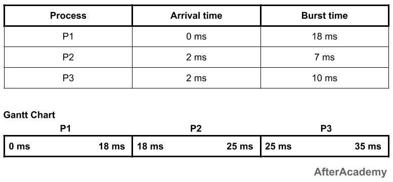
In the above example, you can see that we have three processes P1, P2, and P3, and they are coming in the ready state at 0ms, 2ms, and 2ms respectively. So, based on the arrival time, the process P1 will be executed for the first 18ms. After that, the process P2 will be executed for 7ms and finally, the process P3 will be executed for 10ms. One thing to be noted here is that if the arrival time of the processes is the same, then the CPU can select any process.
---------------------------------------------
| Process | Waiting Time | Turnaround Time  |
---------------------------------------------
|   P1    |     0ms      |      18ms        |
|   P2    |     16ms     |      23ms        |
|   P3    |     23ms     |      33ms        |
---------------------------------------------
Total waiting time: (0 + 16 + 23) = 39ms
Average waiting time: (39/3) = 13ms

Total turnaround time: (18 + 23 + 33) = 74ms
Average turnaround time: (74/3) = 24.66ms
Advantages of FCFS:
- It is the most simple scheduling algorithm and is easy to implement.
Disadvantages of FCFS:
- This algorithm is non-preemptive so you have to execute the process fully and after that other processes will be allowed to execute.
- Throughput is not efficient.
- FCFS suffers from the Convey effect i.e. if a process is having very high burst time and it is coming first, then it will be executed first irrespective of the fact that a process having very less time is there in the ready state.
Shortest Job First (Non-preemptive)
In the FCFS, we saw if a process is having a very high burst time and it comes first then the other process with a very low burst time have to wait for its turn. So, to remove this problem, we come with a new approach i.e. Shortest Job First or SJF.
In this technique, the process having the minimum burst time at a particular instant of time will be executed first. It is a non-preemptive approach i.e. if the process starts its execution then it will be fully executed and then some other process will come.
Example:
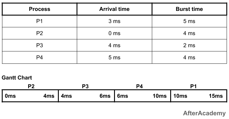
In the above example, at 0ms, we have only one process i.e. process P2, so the process P2 will be executed for 4ms. Now, after 4ms, there are two new processes i.e. process P1 and process P3. The burst time of P1 is 5ms and that of P3 is 2ms. So, amongst these two, the process P3 will be executed first because its burst time is less than P1. P3 will be executed for 2ms. Now, after 6ms, we have two processes with us i.e. P1 and P4 (because we are at 6ms and P4 comes at 5ms). Amongst these two, the process P4 is having a less burst time as compared to P1. So, P4 will be executed for 4ms and after that P1 will be executed for 5ms. So, the waiting time and turnaround time of these processes will be:
---------------------------------------------
| Process | Waiting Time | Turnaround Time  |
---------------------------------------------
|   P1    |     7ms      |      12ms        |
|   P2    |     0ms      |      4ms         |
|   P3    |     0ms      |      2ms         |
|   P4    |     1ms      |      5ms         |
---------------------------------------------
Total waiting time: (7 + 0 + 0 + 1) = 8ms
Average waiting time: (8/4) = 2ms

Total turnaround time: (12 + 4 + 2 + 5) = 23ms
Average turnaround time: (23/4) = 5.75ms
Advantages of SJF (non-preemptive):
- Short processes will be executed first.
Disadvantages of SJF (non-preemptive):
- It may lead to starvation if only short burst time processes are coming in the ready state(learn more about starvation from here).
Shortest Job First (Preemptive)
This is the preemptive approach of the Shortest Job First algorithm. Here, at every instant of time, the CPU will check for some shortest job. For example, at time 0ms, we have P1 as the shortest process. So, P1 will execute for 1ms and then the CPU will check if some other process is shorter than P1 or not. If there is no such process, then P1 will keep on executing for the next 1ms and if there is some process shorter than P1 then that process will be executed. This will continue until the process gets executed.
This algorithm is also known as Shortest Remaining Time First i.e. we schedule the process based on the shortest remaining time of the processes.
Example:
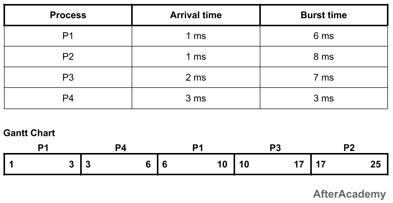
In the above example, at time 1ms, there are two processes i.e. P1 and P2. Process P1 is having burst time as 6ms and the process P2 is having 8ms. So, P1 will be executed first. Since it is a preemptive approach, so we have to check at every time quantum. At 2ms, we have three processes i.e. P1(5ms remaining), P2(8ms), and P3(7ms). Out of these three, P1 is having the least burst time, so it will continue its execution. After 3ms, we have four processes i.e P1(4ms remaining), P2(8ms), P3(7ms), and P4(3ms). Out of these four, P4 is having the least burst time, so it will be executed. The process P4 keeps on executing for the next three ms because it is having the shortest burst time. After 6ms, we have 3 processes i.e. P1(4ms remaining), P2(8ms), and P3(7ms). So, P1 will be selected and executed. This process of time comparison will continue until we have all the processes executed. So, waiting and turnaround time of the processes will be:
---------------------------------------------
| Process | Waiting Time | Turnaround Time  |
---------------------------------------------
|   P1    |     3ms      |      9ms         |
|   P2    |     16ms     |      24ms        |
|   P3    |     8ms      |      15ms        |
|   P4    |     0ms      |      3ms         |
---------------------------------------------
Total waiting time: (3 + 16 + 8 + 0) = 27ms
Average waiting time: (27/4) = 6.75ms

Total turnaround time: (9 + 24 + 15 + 3) = 51ms
Average turnaround time: (51/4) = 12.75ms
Advantages of SJF (preemptive):
- Short processes will be executed first.
Disadvantages of SJF (preemptive):
- It may result in starvation if short processes keep on coming.
Round-Robin
In this approach of CPU scheduling, we have a fixed time quantum and the CPU will be allocated to a process for that amount of time only at a time. For example, if we are having three process P1, P2, and P3, and our time quantum is 2ms, then P1 will be given 2ms for its execution, then P2 will be given 2ms, then P3 will be given 2ms. After one cycle, again P1 will be given 2ms, then P2 will be given 2ms and so on until the processes complete its execution.
It is generally used in the time-sharing environments and there will be no starvation in case of the round-robin.
Example:
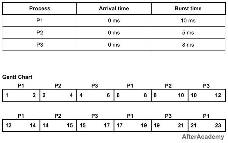
In the above example, every process will be given 2ms in one turn because we have taken the time quantum to be 2ms. So process P1 will be executed for 2ms, then process P2 will be executed for 2ms, then P3 will be executed for 2 ms. Again process P1 will be executed for 2ms, then P2, and so on. The waiting time and turnaround time of the processes will be:
---------------------------------------------
| Process | Waiting Time | Turnaround Time  |
---------------------------------------------
|   P1    |     13ms     |      23ms        |
|   P2    |     10ms     |      15ms        |
|   P3    |     13ms     |      21ms        |
---------------------------------------------
Total waiting time: (13 + 10 + 13) = 36ms
Average waiting time: (36/3) = 12ms

Total turnaround time: (23 + 15 + 21) = 59ms
Average turnaround time: (59/3) = 19.66ms
Advantages of round-robin:
- No starvation will be there in round-robin because every process will get chance for its execution.
- Used in time-sharing systems.
Disadvantages of round-robin:
- We have to perform a lot of context switching here, which will keep the CPU idle(learn more about context switching from here).
Priority Scheduling (Non-preemptive)
In this approach, we have a priority number associated with each process and based on that priority number the CPU selects one process from a list of processes. The priority number can be anything. It is just used to identify which process is having a higher priority and which process is having a lower priority. For example, you can denote 0 as the highest priority process and 100 as the lowest priority process. Also, the reverse can be true i.e. you can denote 100 as the highest priority and 0 as the lowest priority.
Example:
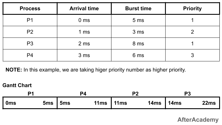
In the above example, at 0ms, we have only one process P1. So P1 will execute for 5ms because we are using non-preemption technique here. After 5ms, there are three processes in the ready state i.e. process P2, process P3, and process P4. Out to these three processes, the process P4 is having the highest priority so it will be executed for 6ms and after that, process P2 will be executed for 3ms followed by the process P1. The waiting and turnaround time of processes will be:
---------------------------------------------
| Process | Waiting Time | Turnaround Time  |
---------------------------------------------
|   P1    |     0ms      |       5ms        |
|   P2    |     10ms     |       13ms       |
|   P3    |     12ms     |       20ms       |
|   P4    |     2ms      |       8ms        |
---------------------------------------------
Total waiting time: (0 + 10 + 12 + 2) = 24ms
Average waiting time: (24/4) = 6ms

Total turnaround time: (5 + 13 + 20 + 8) = 46ms
Average turnaround time: (46/4) = 11.5ms
Advantages of priority scheduling (non-preemptive):
- Higher priority processes like system processes are executed first.
Disadvantages of priority scheduling (non-preemptive):
- It can lead to starvation if only higher priority process comes into the ready state.
- If the priorities of more two processes are the same, then we have to use some other scheduling algorithm.
Multilevel Queue Scheduling
In multilevel queue scheduling, we divide the whole processes into some batches or queues and then each queue is given some priority number. For example, if there are four processes P1, P2, P3, and P4, then we can put process P1 and P4 in queue1 and process P2 and P3 in queue2. Now, we can assign some priority to each queue. So, we can take the queue1 as having the highest priority and queue2 as the lowest priority. So, all the processes of the queue1 will be executed first followed by queue2. Inside the queue1, we can apply some other scheduling algorithm for the execution of processes of queue1. Similar is with the case of queue2.
So, multiple queues for processes are maintained that are having common characteristics and each queue has its own priority and there is some scheduling algorithm used in each of the queues.
Example:
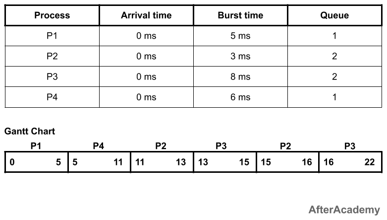
In the above example, we have two queues i.e. queue1 and queue2. Queue1 is having higher priority and queue1 is using the FCFS approach and queue2 is using the round-robin approach(time quantum = 2ms).
Since the priority of queue1 is higher, so queue1 will be executed first. In the queue1, we have two processes i.e. P1 and P4 and we are using FCFS. So, P1 will be executed followed by P4. Now, the job of the queue1 is finished. After this, the execution of the processes of queue2 will be started by using the round-robin approach.
Multilevel Feedback Queue Scheduling
Multilevel feedback queue scheduling is similar to multilevel queue scheduling but here the processes can change their queue also. For example, if a process is in queue1 initially then after partial execution of the process, it can go into some other queue.
In a multilevel feedback queue, we have a list of queues having some priority and the higher priority queue is always executed first. Let's assume that we have two queues i.e. queue1 and queue2 and we are using round-robin for these i.e. time quantum for queue1 is 2 ms and for queue2 is 3ms. Now, if a process starts executing in the queue1 then if it gets fully executed in 2ms then it is ok, its priority will not be changed. But if the execution of the process will not be completed in the time quantum of queue1, then the priority of that process will be reduced and it will be placed in the lower priority queue i.e. queue2 and this process will continue.
While executing a lower priority queue, if a process comes into the higher priority queue, then the execution of that lower priority queue will be stopped and the execution of the higher priority queue will be started. This can lead to starvation because if the process keeps on going into the higher priority queue then the lower priority queue keeps on waiting for its turn.
This is all about process scheduling algorithms. That's it for this blog. Hope you learned something new today.
Do share this blog with your friends to spread the knowledge. Visit our YouTube channel for more content. You can read more blogs from here.
Keep Learning 🙂
Team AfterAcademy!
Written by AfterAcademy Tech
Share this article and spread the knowledge
Read Similar Articles
AfterAcademy Tech
What is a Process in Operating System and what are the different states of a Process?
In this blog, we will learn about Process in Operating System and we will also learn about the various states of a Process during its life cycle.
AfterAcademy Tech
What is an Operating System and what are the goals and functions of an Operating System?
In this blog, we will learn what an Operating System is and what are the goals of an Operating System. We will also learn the functionalities of an Operating System that helps in achieving the goal of the OS.

AfterAcademy Tech
What is Process Synchronization in Operating System?
In this blog, we will learn about Process Synchronization in Operating System. Process Synchronization is used to deal with critical section problem.
AfterAcademy Tech
Process Control Block in Operating System
In this blog, we will learn about Process Control Block also known as PCB and we will see various attributes that are present in the Process Control Block.