Mastering Backpropagation in Neural Network
AfterAcademy Tech
•
25 Nov 2019

In this article, we are going to learn one of the most important Machine Learning Algorithm which is Backpropagation in Neural Network in the simplest way ever.
In this blog, we are going to cover the following topics to master the Backpropagation:
- Intuition behind Backpropagation
- Basics of Neural Network
- Why the Backpropagation Algorithm?
- Forward Propagation
- Backpropagation Algorithm with Derivation
- Putting up all things together
Intuition behind Backpropagation:
Let's feel in a Backpropagation way. Think of a situation where we are playing against an elite grandmaster chess player. We are badly defeated by him but the grandmaster allowed us to undo our steps and rectify the errors made during the game. After going through all the previous steps, we rectified most of our errors. Now, the game was a little more competitive and our performance was better than the previous one but we were defeated again. We again undo the steps and corrected our errors. We repeat these steps until we finally defeated that player. This is what Backpropagation does. Backpropagation moves backward from the derived result and corrects its error at each node of the neural network to increase the performance of the Neural Network Model.
The goal of Backpropagation is to optimize the weights so that the neural network can learn how to correctly map arbitrary inputs to outputs.
Basics of Neural Network:
Every human has a general question of how our brains work? How these neurons are working together and making one of the most complex things in the universe which is our brain?
There are trillions of the neurons connected and each neuron act as a node of a network. The input collected from our sense organs is fed as an input to the network of neurons which generates the output after passing it through different neuron layers.
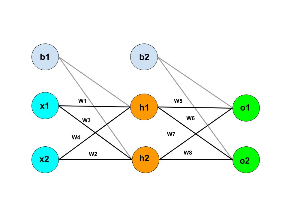
We use the same concept in Neural Network. In Neural Network, there are layers of nodes that act as an activation unit between input and output. Let's visualize it with the help of diagram:

Here, x1 and x2 are the input of the Neural Network. h1 and h2 are the nodes of the hidden layer. o1 and o2 displays the number of outputs of the Neural Network. b1 and b2 are the bias node.
Why the Backpropagation Algorithm?
Backpropagation Algorithm works faster than other neural network algorithms. If you are familiar with data structure and algorithm, backpropagation is more like an advanced greedy approach. The backpropagation approach helps us to achieve the result faster. Backpropagation has reduced training time from month to hours. Backpropagation is currently acting as the backbone of the neural network.
Forward Propagation
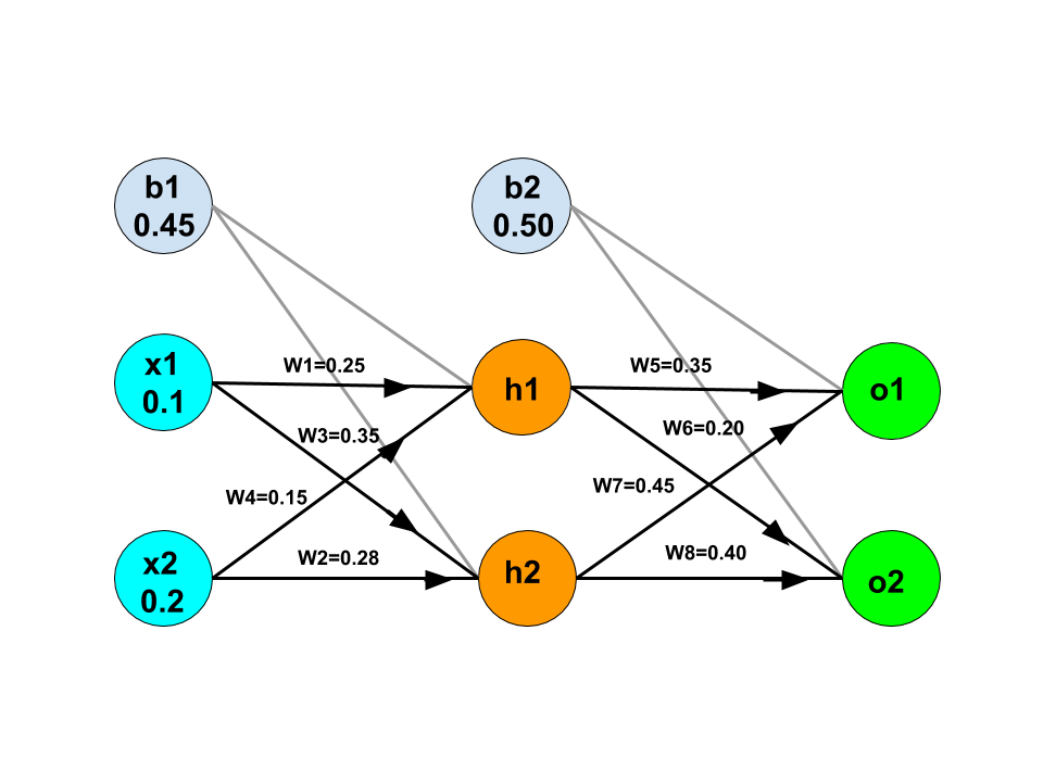
In forward propagation, we generate the hypothesis function for the next layer node. The process of generating hypothesis function for each node is the same as that of logistic regression. Here, we have assumed the starting weights as shown in the below image.

Now, let's discuss how to generate the correct value of nodes and the weight of the edge to get the more accurate output.
As we are going to derive the equation and do some nice calculations. The best way to grasp all the things completely is to calculate each value by ourselves as we go along with the blog. We can take a pen, paper, calculator and start now.
The correct output from output node o1 and o2 be y1 and y2 respectively. Let's assume the value of y1 = 0.05 and the value of y2 = 0.95 which are the correct outputs labeled for the given inputs.
Here, the values of h1 and h2 can be calculated as below:
h1 = w1 * x1 + w4 * x2 + b1
h1 = 0.25 * 0.1 + 0.15 * 0.2 + 0.45 = 0.505
h2 = w3 * x1 + w2 * x2 + b1
h2 = 0.35 * 0.1 + 0.28 * 0.2 + 0.45 = 0.541
If we use the sigmoid function as the activation function, then the value of the output of h1 is :

H(h1) is the final output of node h1 which is equal to 0.623633
Similarly, the value of H(h2) can be calculated as 0.632045
The output of the node can be calculated as below:
o1 = w5 * H(h1) + w6 * H(h2) + b2
o1 = 0.35 * 0.623633 + 0.20 * 0.632045 + 0.5 = 0.794609
o2 = w7 * H(h1) + w8 * H(h2) + b2
o2 = 0.45 * 0.623633 + 0.40 * 0.632045 + 0.5 = 1.0334528
Then, we apply the activation function and store it in the output node.

After the final activation function, the values of out(o1) is 0.6888201 and the out(o2) is 0.7375445. Till now, we have done Forward Propagation only, now let's jump into the Backpropagation.
Backpropagation Algorithm with Derivation
The Backpropagation algorithm has the goal to update each weight of the algorithm so that the total error gets reduced. We start from the weights connecting the output node and move towards the input node which means we move backward.
Many predefined functions implement this algorithm. For practical use, we can directly call the function and implement a neural network. For the sake of knowledge, let's move towards its mathematical derivation.
The total squared error of the neural network can be written like below:

Here, y1 and y2 are target outputs that are expected from the node o1 and o2.
If we put all the values, we get the total error as 0.22661423.
Now, we need to go backward from the output node and change the weight such that the total squared error can get changed by it. Here, for example, for the weight w5, we need to calculate the partial derivative of the total error with respect to w5, as we want to see the change in total error with respect to change in w5. Since there is no direct relation between w5 and E(total) from the above equations, so we will try to differentiate E(total) by the variable which is dependent on it. We figured out E(total) depends on out(o1) which depends on net-input on o1. The net-input depends on the value of w5. Applying the chain rule, we get:

Here net(o1) means the net input that is being received by the o1 output node. After receiving the net input, net(o1), the output node applies activation function on it and out(o1) is stored as output.
Let's see each component of the chain product and find its value. The change in total error with respect to output o1 is:


Since out(o1) is a sigmoid function that depends on net(o1). Now, we will find out the change in output in o1 which is out(o1) with respect to net-input in o1 node:


The only partial differential left is the change in net-input in o1 with respect to w5:


Putting all the value of the above three equation in chain rule, we get:


From the above, we can conclude that a decrease in w5 can lead to a decrease in total error. To optimize the value of w5, we need to change the value of w5 at a specific rate such that change in w5 will not cause an increase in total error.
To change the value of weight w5, we add it by the partial differential of total error by w5 multiplied by learning rate of 0.5:


Similarly, we will change the weights of all edges connected to the output edge of the Neural network. After optimizing the weights w6, w7, and w8 to reduce the total error, we move to the computation of weights connecting the input layer with the hidden layer. Let's calculate the new value of weight w1.
So, we need to calculate the partial derivative of the total error with respect to w1, as we want to see the change in total error with respect to change in w1. Applying the chain rule, we get:

Let's calculate the change in total error with respect to out(h1). For easier calculation, lets break E(total) into E(o1) and E(o2). We know the E(o1) is an error in o1 node and E(o2) is an error in the o2 node.

We know error in o1 node does not directly depend on out(h1). The net-input of o1 depends on the output of h1. So, again applying the chain rule.
Give numbers to all of your equations for better understanding.
At first, we will calculate error in o1 with respect to out(h1):

As we know the values of some part of the differential equation while solving w5. So, we simply put the value and calculate the equation.

We know the equation of net(o1) which is net-input in h1 while solving the Forward Propagation, so we can differentiate it with respect to out(h1).

Putting the value of the above two equations to get the change in the error of o1 with respect to out(h1), we get:

Similarly, we calculate the change in the error of o2 with respect to out(h1).

Using the value of the above two equations to get the value of the change in the total error with respect to out(h1).

Our first differential equation of the RHS side of the chain rule is calculated. Now we will calculate differential of out(h1) w.r.t net-input of h1. We know out(h1) is a sigmoid function, so its equation is:

Differentiating it w.r.t net(h1), as, we already know out(h1), we can calculate the value like below:

We know the formula of net(h1) from the Forward Propagation which is:

Differentiating it w.r.t w1, we get:

Putting all these equations to get change in total error w.r.t change in weight of w1, we get:

The negative change in total error w.r.t w1 indicates that we need to reduce the value of w1 to minimize the error.
Now, we subtract w1 with the change in total error with respect to w1 at a specific learning rate of 0.5.

The final value of w1 will be 0.249921
Similarly, we will calculate w1, w2, w3, and w4. And, we again calculate the total error. We can calculate the total error and check that previously it was 0.22661423 and now it is decreased to 0.224991003. Though this change might look not so effective, after thousands of iterations, the error will be less than 0.1.
Putting up all things together
Now, how to use all of these together and train our model. So, here are the steps to train the Neural Network:
- Initialize the weights of the Neural Network.
- Apply the Forward Propagation to get the activation unit value.
- Implement the Backpropagation to compute the partial derivative.
- Repeat the Backpropagation for n number of times till you minimize the error.
Here, we have done the above derivation and calculation for mastering the Backpropagation. But, we can use the Machine Learning library for training the model using Backpropagation as the library already implements the Backpropagation Algorithm for us.
I hope we have got the idea of Backpropagation, how it works, and its intuition.
Thank you so much for your time.
Happy Machine Learning 🙂
Team AfterAcademy
Written by AfterAcademy Tech
Share this article and spread the knowledge
Read Similar Articles
AfterAcademy Tech
Mastering Activation Functions in Neural Networks
In this blog, we are going to learn what is activation function and it's types. We will also learn what is a good Activation function and when to use which Activation function in Neural Network.

AfterAcademy Tech
What is a network and what are the nodes present in a network?
In this blog, we will mainly learn about a computer network and its node. We will also cover the classification, goals, and applications of a computer network.

AfterAcademy Tech
What is network topology and types of network topology?
In this blog, we will learn about various network topologies, their advantages and disadvantages in a computer network.

AfterAcademy Tech
What are Peer-to-Peer networks and Server-Based networks?
In this blog, we will learn about the types of network based on design, that are Peer-to-Peer, and Server-Based networks. We will also see the applications, advantages, and disadvantages of using these networks.
