Idea of Dynamic Programming

The Idea for this blog is to discuss the new algorithm design technique which is called Dynamic Programming. This is an important approach to problem-solving in computer science where we use the idea of time-memory trade-off to improve efficiency. Even many tech companies like to ask DP questions in their interviews. In this blog, we will be exploring the following concepts items related to DP:

• Recursive solution of finding nth Fibonacci
• Improving efficiency using time memory trade-off
• Top-Down Implementation (Memoization)
• Bottom-Up Implementation (Tabulation)
• Comparison: Top-Down vs Tabulation
• Critical concepts to explore further
• Suggested problems to solve

Let’s first discuss the problem of finding nth Fibonacci.

Problem Statement: Find nth Fibonacci number where a term in Fibonacci is represented as

F(n) = F(n-1) + F(n-2), where F(0) = 0 and F(1) = 1

Solution Idea: Recursive Approach

We can solve the problem recursively with the help of the above recurrence relation. Here we are solving the problem of size n using the solution of sub-problem of size (n-1) and size (n-2), where F(0) and F(1) are the base cases.

Pseudo Code

int fib(n)
{
    if(n == 0)
        return 0
    else if(n == 1)
        return 1
    else
        return fib(n-1) + fib(n-2)
}

Complexity Analysis

The above code looks simple in the first look but it is really inefficient. Let's analyse it and understand the reason for its inefficiency.

Here is the recursion tree diagram

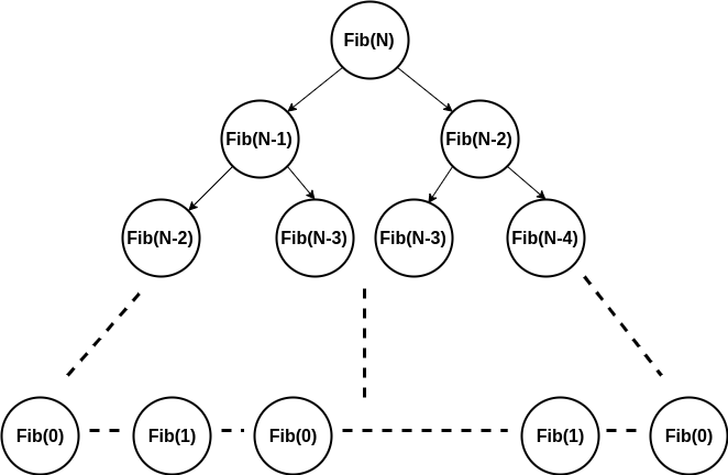
In the recursion tree method, The total number of recursive calls = Total number of nodes in the recursion tree.

Similarly, if we have k level in the recursion tree, then the total number of operations performed by recursion = L1 + L2 + L3 ......Lk, where any Li is the total number of operations at the ith level of the recursion tree.

If we observe closely then we can list down the following things:

• We are doing O(1) operation at each recursive call.
• The total number of recursive calls are growing exponentially, as we move downward in the tree i.e. 2, 4, 8, 16...and so on.
• The height of each leaf node is in the range of (n/2, n). So we can say that the total height of the recursion tree = O(n) = cn, where c is some constant. (Think!)

Total number of recursive calls = 1 + 2 + 4 + 8 ...+ 2^cn

= (2^cn - 1) / (2 - 1) (Using the summation formula of geometric series)

= O(2^n)

Time Complexity = O(2^n). This is an inefficient algorithm because time complexity is growing exponentially with respect to the input size(n). Overall, It will take a very long time to generate output for a small value of n like 30 or 50 or 70.

Critical question: why the time complexity of this recursive solution is growing exponentially?

Let’s explore the reason with the help of the recursion tree for finding the 5th Fibonacci.

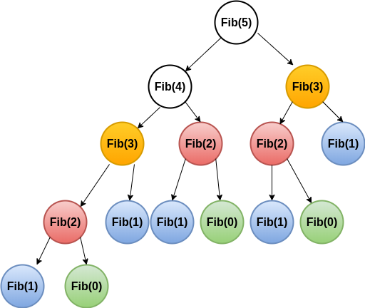
From the above diagram, we are solving the same sub-problems again and again during the recursion i.e. Fib(3) is calculated 2 times, Fib(2) is calculated 3 times and so on. If we further increase the value of n then repeated sub-problems will also increase. Because of the repeated solution of the same sub-problem, our time complexity is in the exponential order of n. Note: There are only n+1 different subproblems in the above recursion. (Think!)

Critical Question: Can we stop the repeated computation and improve the efficiency of the solution?

The Idea of Dynamic Programming

Rather than computing the same sub-problem, again and again, we can store the solution of these sub-problems in some memory, when we encounter this sub-problem first. When this sub-problem appears again during the solution of other sub-problem, we will return the already stored solution in the memory. This is a wonderful idea of Time-Memory Trade-Off, where we are using extra space to improve the time complexity. (Think!)

Let's discuss the efficient solution using the dynamic programming approach. There are two different ways of solving Dynamic programming problems:

• Memoization: Top Down
• Tabulation: Bottom Up

Let's understand these two terms:

• Top-down: This is a modified version of the above recursive approach where we are storing the solution of sub-problems in an extra memory or look-up table to avoid the recomputation.
• Bottom-up: This is an iterative approach to build the solution of the sub-problems and store the solution in an extra memory.

Solution Idea: Top-down Approach (Memoization)

Solution Steps

1. We can use a global array or a lookup table of size N+1 to store the solution of the different sub-problems. let's say F[N+1].
2. Initialize all the values in the array to -1(As the value of Fibonacci can’t be negative). This could help us to check whether the solution of the sub-problem has been already computed or not.
3. We can do the following modification in the recursive solution:

• If(F[N] < 0), it means the value of Fibonacci of N has not been computed yet. We need to calculate the solution recursively and store it at the Nth index of the table F[N] = fib(N-1) + fib(N-2).
• If (F[N] > 0), then just return the value stored at F[N] (Because we have already computed the F[N] during the recursion).
• N= 0 and N=1 are the base cases because we already know the value for this and we can directly store the solution at F[0] and F[1].

Pseudo Code

Initaize an array F[N+1] with negative values.
int fib(N)
{
    if( F[N] < 0 )
    {
        if( N <= 1 )
            F[N] = N
        else
            F[N] = fib(N-1) + fib(N-2)
    }
    return F[N]
}

Complexity Analysis

The total number of recursive calls = 2N-1, because we are avoiding recomputations and solving N+1 sub-problems only once. (Think!)

Time Complexity = O(N).

Space Complexity: O(N) for an extra table to store the solution of the subproblems.

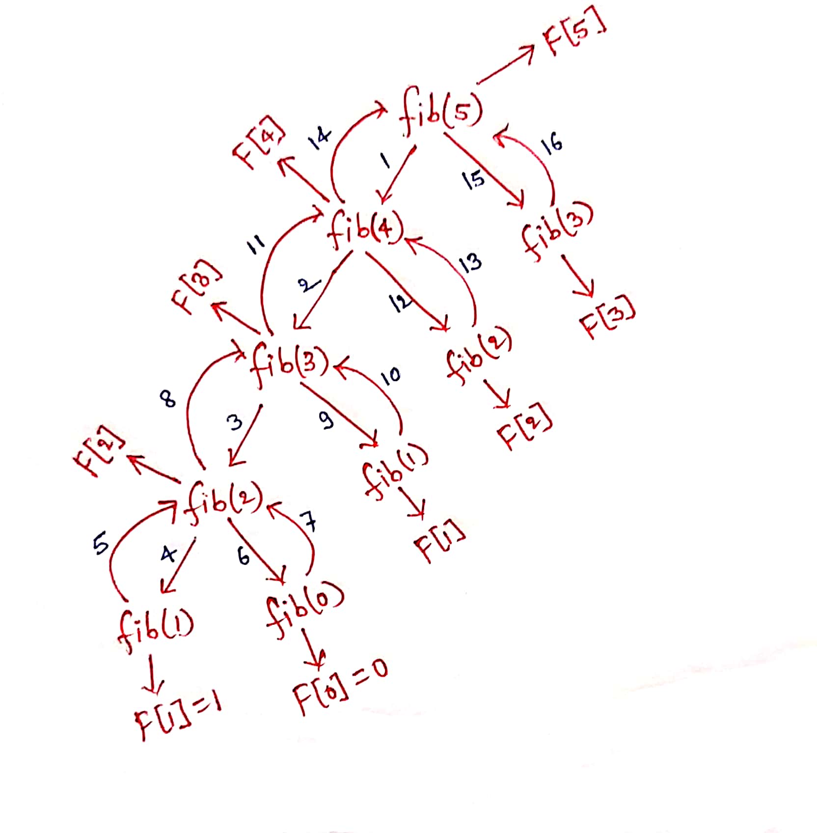
Critical observation

Recursion is coming top-down from the larger problem of size n to the base case of size 0 and 1. But it is storing the results in a bottom-up manner where F[0] and F[1] are the first two values which get stored in the table.

Order of recursive calls: fib(n)-> fib(n-1)-> fib(n-2) ...-> fib(i)-> fib(i-1)-> fib(i-2)...-> fib(2)-> fib(1)-> fib(0)

Order of storing the results in the table: F[0]-> F[1]-> F[2] ...-> F[i]-> F[i-1]-> F[i-2]...-> F[n-2]-> F[n-1] ->F[n]

If you draw the recursion tree for n=5, then it looks like this

Critical question: So rather than using the complex recursive approach, can we just use a simple iterative approach to store the results in the table? or can we build the solution from base case of size 0 and 1 to the larger problem of size n?

Solution Idea: Bottom-up Approach(Tabulation)

In this approach, we are solving the smaller problems first and then combining the results of smaller problems to get the solution of the larger problem of the size n.

Solution steps

1. Define Table Structure and Size: To store the solution of smaller sub-problems in a bottom-up approach, we need to define the table structure and its size.

• Table Structure: The table structure is defined by the number of problem variables. Here we have only one variable on which the state of the problem depends i.e. which is n here. (The value of n is decreasing after every recursive call). So, we can construct a one-dimensional array to store the solution of the sub-problems.
• Table Size: The size of this table is defined by the total number of different subproblems. If we observe the recursion tree, there can be total (n+1) sub-problems of different sizes. (Think!)

2. Initialize the table with the base case: We can initialize the table by using the base cases. This could help us to fill the table and build the solution for the larger sub-problem. F[0] = 0 and F[1] = 1

3. Iterative Structure to fill the table: We should define the iterative structure to fill the table by using the recursive structure of the recursive solution.

Recursive Structure: fib(n) = fib(n-1) + fib(n-2)

Iterative structure: F[i] = F[i-1] + F[i-2]

4. Termination and returning final solution: After storing the solution in a bottom-up manner, our final solution gets stored at the last Index of the array i.e. return F[N].

Pseudo Code

int F[N+1] // array(memory to store results)
int fib(int N)
{
    F[0] = 0 // base cases
    F[1] = 1 // base cases
    
    for( i = 2 to N )
        F[i] = F[i-1] + F[i-2]
    
    return F[N]
}

Complexity Analysis

We are using a table of size N+1 and running only one loop to fill the table. Time Complexity = O(N), Space Complexity = O(N)

Comparison: Memoization vs Tabulation

• Ease of Coding - Memoization is easy to code i.e. you just add an array or a lookup table to store down the results and never recomputes the result of the same problem. But in the tabulation, you have to come up with ordering or iterative structure to fill the table.
• Speed - Memoization can be slower than tabulation because of large recursive calls.
• Stack Space - With memoization, if the recursion tree is very deep, you will run out of stack space, which will crash your program.
• Subproblem Solving - In Tabulation, all subproblems must be solved at least once but in Memoization, all problems need not be solved at all, the memoized solution has the advantage of solving those sub-problems that are definitely required.

Critical Ideas to explore further

• How to recognize a DP problem? or What type of questions can be solved using the idea of DP?
• What are the optimization and combinatorial problems? A variety of optimization and combinatorial problems can be solved using the idea of dynamic programming.
• What is an optimal sub-structure property in a DP problem?
• Can we recognize some common steps or patterns involved in the solution of a DP problem? We always recommend learners to practice and learn different patterns to solve the problem recursively and fill the table iteratively.
• Designing the recursive solution of a DP problem is logical art! Explore the recursive solution of some famous DP problems.
• Why should we prefer a bottom-up approach for the implementation? In a bottom-up approach, We advise learners to always take care of table structure, table size, table initialization, iterative structure and termination condition.
• Comparison between Dynamic Programming and Divide and Conquer Approach
• Comparison between Dynamic Programming and Greedy Approach

Suggested Problems to solve in Dynamic Programming

• Finding n-th Fibonacci number
• Count of different ways to express N
• Longest Common Subsequence
• Rod Cutting Problem
• Longest Palindromic Subsequence

Happy coding! Enjoy Algorithms.