Getting started with Tensorflow 2.0 Tutorial - Step by step Guide

Tensorflow is an awesome open-source deep-learning library for everyone. Now that Tensorflow 2.0 has been released. There are many great features available in 2.0. Tensorflow 2.0 is a major upgrade to Tensorflow 1.x. In this blog post, we will go through the step by step guide on how to use Tensorflow 2.0 for training the model in Machine Learning. This blog is for both beginners as well as for advanced users who want to get started with Tensorflow 2.0 for Machine Learning.

In this blog, we are going to cover the following topics:

• Why Tensorflow 2.0?
• Installation of Tensorflow 2.0
• Using it with Jupyter Notebook
• Using it in Google Colab
• Components of Tensorflow 2.0
• Beginners approach for training a Machine Learning model
• Advanced approach for training a Machine Learning model
• Multiple GPU distribution strategy
• Saving a model
• Some customizations in Tensorflow 2.0

Why Tensorflow 2.0?

Tensorflow 2.0 is released so that it can be easily used by both beginners and experts. Things that make Tensorflow 2.0 better than other libraries of Machine Learning include:

• Easier to learn.
• Easier to use: You don’t need to worry about the complex syntax because Tensorflow 2.0 has simple syntax which is easy to use.
• Simple yet powerful: The simple syntax doesn't make Tensorflow 2.0 less powerful. Advanced users can do many things with the Tensorflow like, customizing it according to the need, inheriting it and building on top of it for a specific use-case.
• APIs are more familiar for Python developers.
• Keras is now the recommended high-level API: The raw Tensorflow and Keras layers are now integrated which is easy to use and the productivity of the developer is increased.
• Data access is more easy with the expansion of TF datasets.
• Regular python with eager execution by default: If you are new to Tensorflow, then this might sound unfamiliar to you but don’t worry. In Tensorflow 1.x, if we perform the addition of two constant directly then, it doesn’t give us the required arithmetic result instead we have to perform the action inside a session but we can do it directly in Tensorflow 2.0. This is called eager execution. In Tensorflow 1.x, the code is written like:

a = tf.constant(5)
b = tf.constant(3)
c = a * b
with tf.Session() as sess:
  print(sess.run(c))

But due to eager execution, Tensorflow 2.0 has simplified the code.

a = tf.constant(5)
b = tf.constant(3)
c = a * b
print(c)

• More complete low-level APIs: We can inherit and build on top of the internal of Tensorflow. The new APIs of Tensorflow 2.0 gives more control to us.

Installation of Tensorflow 2.0

• Install Python of version 3.4+ which is a prerequisite.

Check the python version of the system by following code on the command prompt.

 $  python --version

If not upgraded, upgrade it as follows:-

python -m pip install --upgrade pip

• Write the following code in the command prompt to install Tensorflow using pip.

pip install tensorflow

• Test the installed Tensorflow by opening the python ide and writing this code:-

import tensorflow as tf 

If there is no error, then the Tensorflow is installed properly.

Using Tensorflow 2.0 with Jupyter notebook?

To use Tensorflow2.0 on Jupyter notebook, we need to follow these steps:-

1. Install Anaconda. Download Anaconda for the platform and choose the Python 3.4+ version: https://www.anaconda.com/download
2. Open Anaconda Navigator and create an environment by clicking create on the environment section.
3. Goto not installed tab in the environment section at top of the list of libraries and search Tensorflow.
4. Click on Tensorflow and apply it.
5. After the process is completed, open the Jupyter notebook and then write the following code to check if Tensorflow is installed properly or not.

import tensorflow as tf 

If there is no error, then the TensorFlow is installed properly.

Using Tensorflow 2.0 with Google Colab?

Google Colab is a free cloud service that supports free GPU where we can develop Machine Learning programs and improve our Python skills. We can use Tensorflow2.0 with Google Colab by following steps:-

1. Open Google Colab on the link. https://colab.research.google.com/
2. Create a notebook of python 3.
3. Connect to GPU/CPU.
4. Check the version of Tensorflow, if it is not 2.0 then uninstall Tensorflow using

!pip uninstall tensorflow

And then install it by

!pip install tensorflow

Components of Tensorflow 2.0

• Dataset: Tensorflow 2.0 provides a collection of the dataset which can be downloaded and used for implementing the Machine Learning model. It handles downloading and preparing the data and constructing a tf.data.Dataset for us.

"""To import tensorflow_datasets package."""
import  tensorflow_datasets as tfds
"""tfds.load is used to load the dataset from tensorflow_dataset.
After this, dataset will start to download unless you specify download=False"""
mnist_train = tfds.load(name="mnist", split="train")

• API: We can access the Keras APIs which are implemented in Tensorflow 2.0 through tf.keras. In Keras, we assemble layers to build a model and the most common stack of the layer is tf.keras.sequential.

model = tf.keras.models.Sequential([
  tf.keras.layers.Flatten(input_shape=(28, 28)),
  tf.keras.layers.Dense(128, activation='relu'),
  tf.keras.layers.Dropout(0.2),
  tf.keras.layers.Dense(10, activation='softmax')])

To add a dense layer of with 32 units of model, we code it as:

model.add(layers.Dense(32, activation='relu'))

Similarly, Tensorflow 2.0 has different new APIs which are easy to use.

• Model Training: Training the model is the most important task in Machine Learning. Here we take our dataset, generate a function called hypothesis function for which our dataset mostly fits it. Tensorflow 2.0 has APIs which we can use to train our dataset like below.

model.compile(optimizer='adam',loss='sparse_categorical_crossentropy',metrics=['accuracy'])
model.fit(x_train, y_train, epochs=5)

• Saving the model: We can use model.save() to save the model's architecture, weights, and training configuration in a single file/folder in Tensorflow 2.0. Here, the state at which model was saved can be used again from the same state. We will discuss how to save the model in the later part of this blog.
• Deployment: After saving the model, the model can be used on the web, cloud, Android and many more environments. Tensorflow 2.0 has improved its deployment APIs so that the developer can easily use it for deployment purposes.

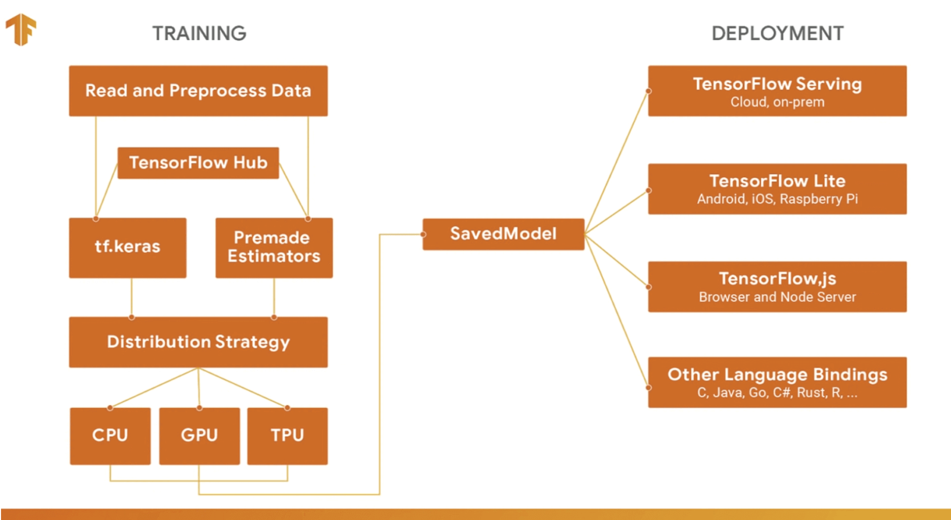
Image Source: Tensorflow Official

Tensorflow is having Tensorflow.js for browser and Tensorflow Lite for mobile platforms.

1. Tensorflow.js: Tensorflow.js(Tensorflow API in Javascript) is an open-source library will help us to develop ml on the browser. In Tensorflow.js, we can run the saved model and predict the output.
2. Tensorflow Lite: Tensorflow Lite is a lightweight version of TensorFlow which can easily run in the mobile platforms and have almost all the features or TensorFlow. Tensorflow Lite is used to deploy the saved ml model on Android, iOS, Raspberry pi.

• Multi GPU: Tensorflow 2.0 provides the simplest way to run on multiple GPUs, on one or many machines. We will discuss it in the later part of this blog.

Beginner approach for training a Machine Learning model

For a beginner, we need to understand how a Machine Learning model is trained. Then, understand which functions or APIs to use to implement the model.

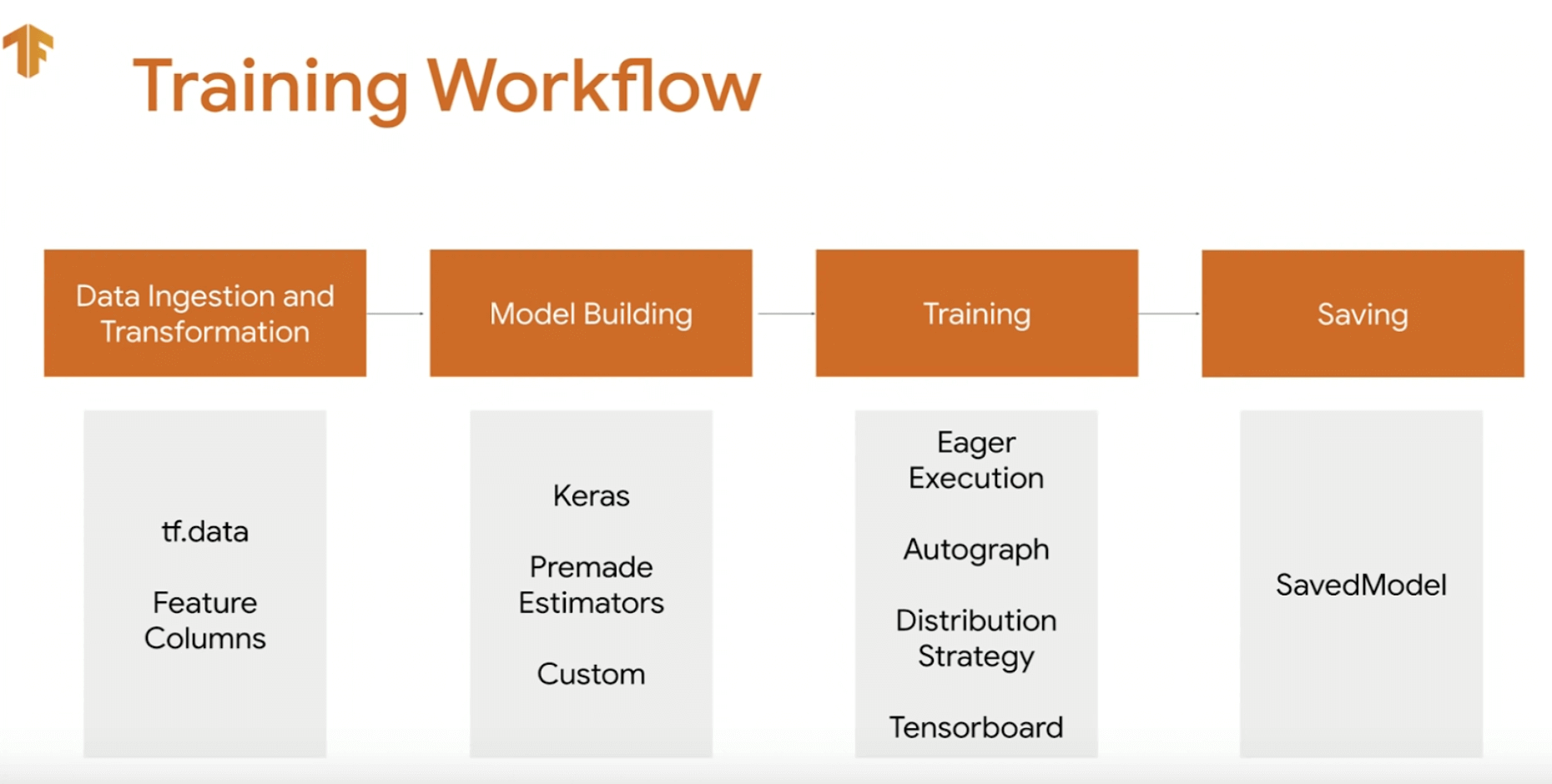
Image Source: Tensorflow Official

1. Data ingestion and Transformation: This is the first step where we are going to train the model. Data ingestion means moving the data from one place to another. Here we move from the data from the TensorFlow dataset to the tensor of our model training. The quality and quantity of data that we gather will directly determine how good our predictive model can be. Data transforming means transforming data from one state to another. Suppose we don’t like the data value of our dataset, then we transform them according to our needs. Here, we prepare our data so that our model can get the perfect fit and perform the best.
2. Model Building: Model building is the phase where we decide which model to use for the given dataset. Suppose we chose a neural network, then we decide how many layers will be there so that the dataset can perfectly fit it. A skeleton of the model is prepared.
3. Training: Training a model aims at creating an accurate model that will predict the most accurate results most of the time. We use the data to incrementally increase the accuracy of our model.
4. Saving: Here the state of the model is saved so that it can be reused again.

import tensorflow as tf
"""The first phase is data ingestion and transformation.
 Here, we take mnist dataset from tensorflow and then split it into training set and test set.
 Training set trains the model and test-set will test how accurate the model is.
 We divide them by 255 because the value of data ranges from 0 to 255.
 Now by dividing it, the range is between 0 to 1."""
mnist = tf.keras.datasets.mnist
(x_train, y_train), (x_test, y_test) = mnist.load_data()
x_train, x_test = x_train / 255.0, x_test / 255.0
"""The code written below describes the model building phase.
 Here we use a sequential layer in the model which means a sequence of the layer.
 Flatten reduces the dimension of the model and dense adds layer of the neuron.
 Each layer needs an activation function which is relu and softmax."""
model = tf.keras.models.Sequential([
  tf.keras.layers.Flatten(input_shape=(28, 28)),
  tf.keras.layers.Dense(128, activation='relu'),
  tf.keras.layers.Dropout(0.2),
  tf.keras.layers.Dense(10, activation='softmax')])
"""Then compile the model with an optimizer and a loss function.
 Then, we train the data so that our dataset gives accurate results.""" 
model.compile(optimizer='adam',loss ='sparse_categorical_crossentropy',metrics=['accuracy'])
model.fit(x_train, y_train, epochs=5)
"""This function gives us how much accurate is our model on the test set."""
model.evaluate(x_test,  y_test, verbose=2)

Advanced approach for training a Machine Learning model

Tensorflow 2.0 provides that flexibility in the code so that we can set the parameter by ourselves and best fit the model. We can shuffle the dataset and then divide them into training and test set by making batches of data.

import tensorflow as tf
from tensorflow.keras.layers import Dense, Flatten, Dropout
from tensorflow.keras import Model
mnist = tf.keras.datasets.mnist
(x_train, y_train), (x_test, y_test) = mnist.load_data()
x_train, x_test = x_train / 255.0, x_test / 255.0
"""10000 is buffer_size, 60000/32 = 1875 is the size of train_ds"""
train_ds = tf.data.Dataset.from_tensor_slices((x_train, y_train)).shuffle(10000).batch(32)
test_ds = tf.data.Dataset.from_tensor_slices((x_test, y_test)).batch(32)

Now, a class is made where the skeleton of the model is prepared.

class MyModel(Model):
    def __init__(self):
        super(MyModel, self).__init__()
        self.flatten = Flatten(input_shape=(28, 28))
        self.dense_1 = Dense(128, activation='relu')
        self.dropout = Dropout(0.2)
        self.dense_2 = Dense(10, activation='softmax')
    def call(self, x):
        x = self.flatten(x)
        x = self.dense_1(x)
        x = self.dropout(x)
        return self.dense_2(x)
model = MyModel()

Here, MyModel class has the details of a layer of the model. Instead of using predefined functions, the object-oriented approach is used to set the parameter of the layers of the model.

loss_object = tf.keras.losses.SparseCategoricalCrossentropy()
optimizer = tf.keras.optimizers.Adam()
"""loss function and optimizer are used for the compiling of the model."""
train_loss = tf.keras.metrics.Mean(name= 'train_loss')
train_accuracy = tf.keras.metrics.SparseCategoricalAccuracy(name='train_accuracy')

test_loss = tf.keras.metrics.Mean(name='test_loss')
test_accuracy = tf.keras.metrics.SparseCategoricalAccuracy(name='test_accuracy')

Gradient tape will show us the variation of weights and biases of each node over a period of time. Gradient Tape tracks the automatic differentiation that occurs during the training. tape.gradient() is used to store the track of all gradients during the training.

@tf.function
def train_step(images, labels):
    with tf.GradientTape() as tape:
        predictions = model(images)
        loss = loss_object(labels, predictions)
    gradients = tape.gradient(loss, model.trainable_variables)
    optimizer.apply_gradients(zip(gradients, model.trainable_variables))
   train_loss(loss)

The training of the model is done by running the training step to the number of epochs. Epochs define the number of times the algorithm will run through the entire dataset. The test-set is set up to predict the accuracy of the result.

@tf.function
def test_step(images, labels):
    predictions = model(images)
    t_loss = loss_object(labels, predictions)
    test_loss(t_loss)
    test_accuracy(labels, predictions)
EPOCHS = 5
for epoch in range(EPOCHS):
    for images, labels in train_ds:
        train_step(images, labels)
    for test_images, test_labels in test_ds:
        test_step(test_images, test_labels)

After training and testing the data, the result of the data is displayed to the user. How the error is varying on the loss function is viewed by the user so that the data doesn’t overfit or underfit the model.

template = 'Epoch {}, Loss: {}, Accuracy: {}, Test Loss: {}, Test Accuracy:{}'
print(template.format(epoch+1,train_loss.result(),train_accuracy.result()*100,test_loss.result(),test_accuracy.result()*100))

Reset the metrics for the next epoch

train_loss.reset_states()
train_accuracy.reset_states()
test_loss.reset_states()
test_accuracy.reset_states()

Multiple GPU distribution strategy

Tensorflow2.0 provides this facility to run our various models over parallel GPUs. The problem is not to get it to work but to use multiple GPUs efficiently. We can either use it for data parallelism, model parallelism or just training different set on the different GPUs. It is easier to set up and saves a lot of time!

Simple code of training a model without multiple GPU is :

model = tf.keras.applications.ResNet50()
optimizer = tf.keras.optimizers.SGD(learning_rate=0.1)
model.compile(..., optimizer=optimizer)
model.fit(train_dataset, epochs=10)

To implement multiple GPU, we need to add only two lines of code like below:

strategy = tf.distribute.MirroredStrategy()
with strategy.scope():
  model = tf.keras.applications.ResNet50()
  optimizer = tf.keras.optimizers.SGD(learning_rate=0.1)
  model.compile(..., optimizer=optimizer)
  model.fit(train_dataset, epochs=10)

tf.distribute.MirroredStrategy supports distributed training on multiple GPUs at the same time. It creates one replica on each GPU and a variable is made in each GPU which is sync with each other. Each GPU gets the data equal to batch size. Taking advantage of multiple GPUs is very easy with Tensorflow 2.0.

Saving a model

Keras provides a safe format using the HDF5 standard. Tensorflow2.0 provides a model.save() function which is used to save the architecture, weights, and training configuration of a model. We can also load them on the web by Tensorflow.js or on Android by TensorFlow lite.
.h5 extension indicates that the model should be saved to the HDF5 file.

model = create_model()
model.fit(train_images, train_labels, epochs=5)
model.save('xyz.h5')

Some customizations in Tensorflow 2.0

Most of the time when the Machine Learning developer is training a model, developers want to change things according to their own needs. Tensorflow 2.0 provides features where we can customize as per our needs. Some of the regularly used customization are:

• Custom callback tools: Callback is a class that is used to provide specific functionality at the time of training or evaluation of Keras model. Callbacks are useful to get a view on internal states and statistics of the model during training.

model.compile(optimizer=Adam(), loss=BinaryCrossentropy(),metrics=[AUC(), Precision(), Recall()])
model.fit(data, epochs=10, validation_data=val_data, callbacks=[EarlyStopping(), TensorBoard(), ModelCheckpoint()])

Here, the callbacks are used in model.fit() method. Here, the class Earlystopping() is used so that the model stops training when the improvement in model is stopped. TensorBoard() class is used for providing a visualization of how the model is getting trained. ModelCheckpoint() is used to save the model after every epoch. Here the model will be saved 10 times.

• Custom activation function: Tensorflow 2.0 provides us extra facilities to either write our own code or customize the existing layer of the model. We can customize the activation function relu in it.

class MyModel(tf.keras.Model):
  def __init__(self, num_classes=10):
    super(MyModel, self).__init__(name='my_model')
    self.dense_1 = layers.Dense(32)
    self.dense_2 = layers.Dense(num_classes,activation='softmax')

def call(self, inputs):
  x = self.dense_1(inputs)
  x = tf.nn.relu(x)
  return self.dense_2(x)

Here, we can use our own custom relu function instead of tf.nn.relu based on requirements. This is how we can do customization in Tensorflow 2.0 according to our requirements.

We have received a good amount of knowledge today.

Thank you so much for your time.

Now, let's start using Tensorflow 2.0 for Machine Learning.

Do share this blog with your fellow developers to spread the knowledge.

Happy Machine Learning 🙂

Team AfterAcademy