Introduction to Arrays

The idea of this blog is to discuss the famous data structure called Array. An Array is one of the important data structures that are asked in the interviews. We will also discuss the idea of the dynamic array and its amortized analysis . In this blog, we will be exploring the following concept items related to the array.

Array- Introduction and Terminologies
Representation of Array
Basic Operations in Array
Idea of Dynamic Array
Amortized Analysis
Suggested problems to solve

Introduction

An array is a collection of items stored at contiguous memory locations. The idea is to store multiple items of the same type together.

It falls under the category of linear data structures. The elements are stored at contiguous memory locations in an array. Most of the algorithms and problem-solving approaches use array in their implementation.

Arrays have a fixed size where the size of the array is defined when the array is initialized.

Terminologies

Two essential terminologies that are used in the array-

Element — Each item stored in an array is called an element.
Index — Each memory location of an element in an array is identified by a numerical index.

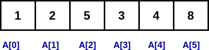
In the above image, [1, 2, 5, 3, 4, 8] are the elements of the array and 0, 1, 2, 3, 4, and 5 are the indexes of the elements of the array.

Representation of Array

Arrays are represented in various ways in different languages. Generally, we need three things to declare an array.

Data Type : Data type of element you want to store in an array.
Name: Name of the array.
Size: Length of the array i.e. how many elements you want to store.

In C language, the array is declared as

data_type name_of_array[size_of_array];

For Example: To store 6 integers in an array we declared it as

int A[6]; // here A is the name of array

In most of the languages, the indexing of array elements starts from 0.

As arrays store elements in contiguous memory locations. This means that any element can be accessed by adding an offset to the base value of the array or the location of the first element. We can access elements as A[i] where "i" is the index of that element.

Basic Operations

There are some specific operations that can be performed or those that are supported by the array. These are:

Traversal : To traverse all the array elements one after another.
Insertion : To add an element at the given position.
Deletion : To delete an element at the given position.
Searching : To search an element(s) using the given index or by value.
Updating : To update an element at the given index.
Sorting: To arrange elements in the array in a specific order.
Merging: To merge two arrays into one.

Traversing

To traverse in an array we use the index property of the array. We can iterate through each element using its index.

void traverse(int A[N])
{
    for(i = 1 to N-1 )
        print(A[i])
}

Insertion

To insert an element item at any position pos, we will shift the array elements from this position to one position forward and will do this for all the elements next to it.

// A is an array
// n is the number of elements in the array
// maxSize is the size of the array
// item is the element to insert
// pos is position at which element will be inserted
void insert(int A[], int n, int maxSize, int item, int pos)
{
    n += 1 // increasing the number of elements
    
    for(i = n; i >= pos; i--)
    {
        A[i] = A[i-1] // shift elements forward
    }
    
    A[pos-1] = item // insert item at pos
}

Deletion

To delete an element at any position pos, we will shift the array elements from this position to one position forward and will do this for all elements next to it.

void delete(int A[], int n, int pos)
{
    for( i = pos-1 to n-2 )
    {
        A[i] = A[i+1] // shift element backwards
    }
    n -= 1 // decreasing size by 1
}

Searching

To search an element in the array, just traverse through the array and check at each position.

bool search(int A[], int n, int item)
{
    for( i = 0 to n-1 )
    {
        if( A[i] == item )
            return true
    }
    return false
}

Updating

To update the value at any index just set the value

void update(int A[], int n, int idx, int val)
{
    A[idx] = val // update the value at that index
}

The Idea of Dynamic Array

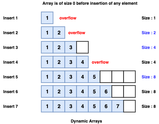
One limitation of arrays is that they’re fixed size, meaning you need to specify the number of elements your array will hold ahead of time. So, here comes the concept of Dynamic Array. A dynamic array expands as you add more elements to it. So you don’t need to determine the size ahead of time. Usually, when the array is full, then the array doubles in size.

Analysis

This additional functionality takes some cost. When we don’t have any space to insert a new element, we allocate a bigger array and copy all the elements from the previous array.

The coping of elements take O(N) time, where N is the number of elements. That is, it is a costly process to append new elements in an array, as compared to normal arrays where insertion takes O(1) time.

But insertion takes O(N) when we insert into a full array and that’s pretty rare. Most of the insertion still takes O(1) and sometimes it will take O(N).

So, focusing on each insertion individually seems a bit harsh. So a fair analysis will be if we look at the cost of a single insertion averaged over a large number of insertion. This is called Amortized analysis.

Amortized Analysis

It is used for analysis of algorithms when the occasional operation(i.e. operations that are very rare) is very slow, but most of the operations are very fast.

Some data structures like Dynamic Arrays, Hash tables, Disjoint sets, etc use amortized analysis for their analysis.

In Amortized Analysis, we analyze a sequence of operations and guarantee that worst-case average time is lower than that of worst-case time of a particular expensive operation.

Let us calculate the time complexity of insertion in a dynamic array using amortized analysis.

Item No      1    2     3    4    5    6   7   8    9   10 .....
Table Size   1    2     4    4    8    8   8   8   16   16 .....
Cost         1  (1+1) (1+2)  1  (1+4)  1   1   1 (1+8)  1  .....

Calculating the total cost,

Total cost = (1 + 1 + 1 + ... {Cost of insertion}) + (1 + 2 + 4 + 8 + ... {cost of re-sizing})

Amortized Cost = Total Cost / No. of Elements.

Amortized Cost = [( 1 + 1 + 1 + … N times) + ( 1 + 2 + 4 .. LogN times)]/N
= (n + 2n)/n    // Sum of G.P for logN terms
= 3

So Amortized Cost = O(1), which is constant time.

The above Amortized analysis is done using the Aggregate Method. There are two more ways to do the Amortized Analysis named Accounting Method and Potential Method.

One more important note is that amortized analysis does not include probability. There is also another different notion of average-case running time where algorithms use randomization to make them faster and expected running time is faster than the worst-case running time. These algorithms are analyzed using Randomized Analysis. Examples of these algorithms are Randomized Quick Sort, Quick Select and Hashing.